Hello


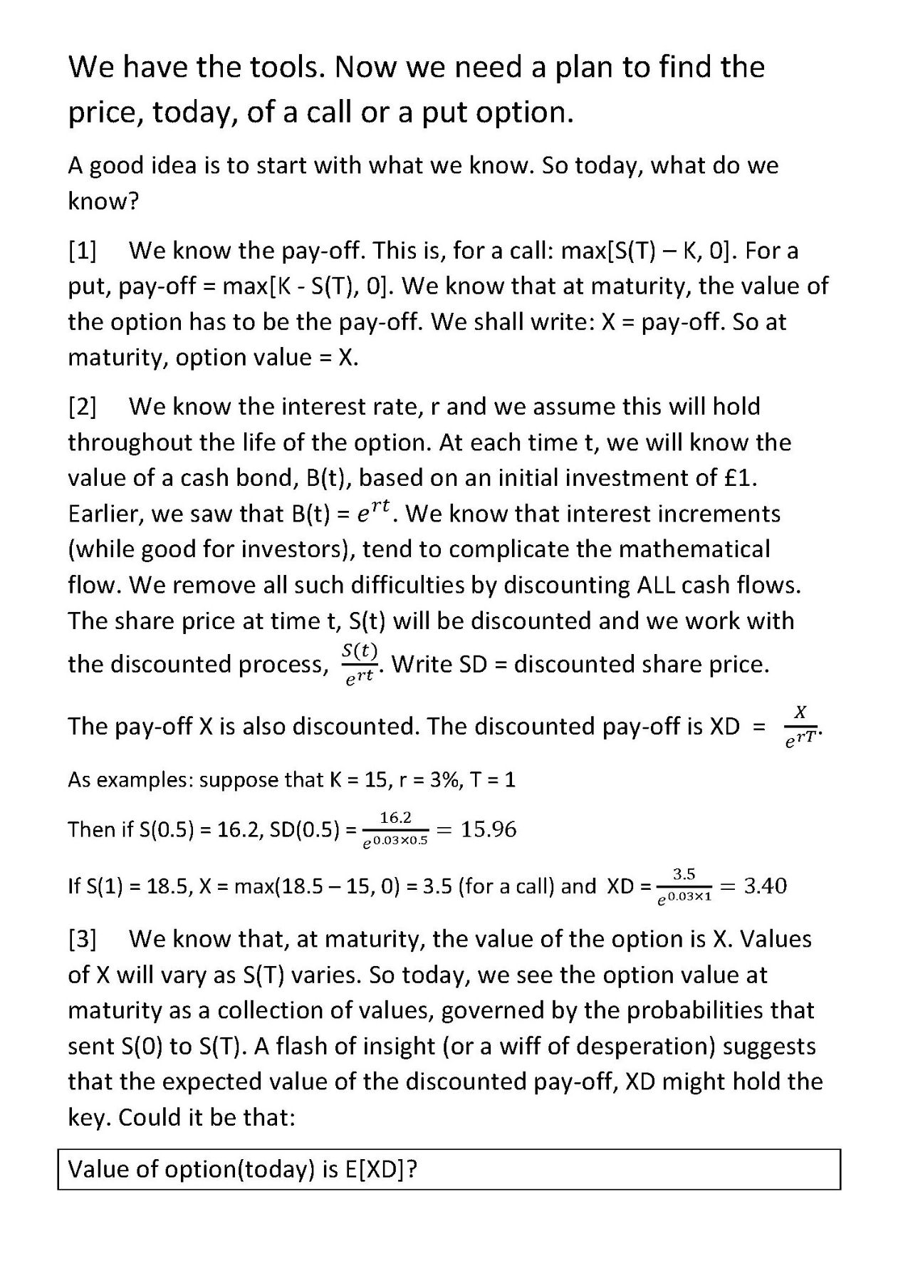
Family
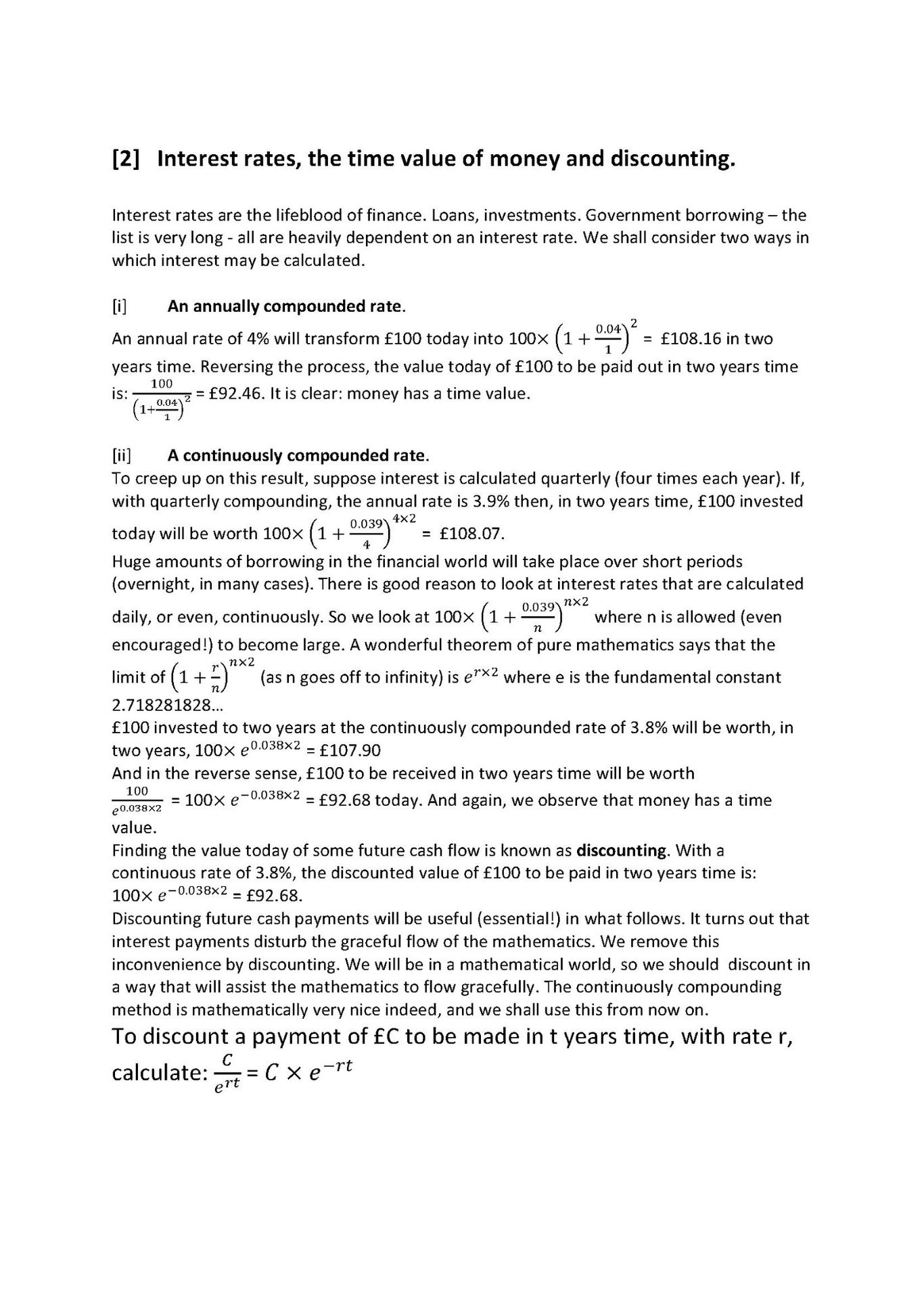
Here they are, with six people who changed my life.


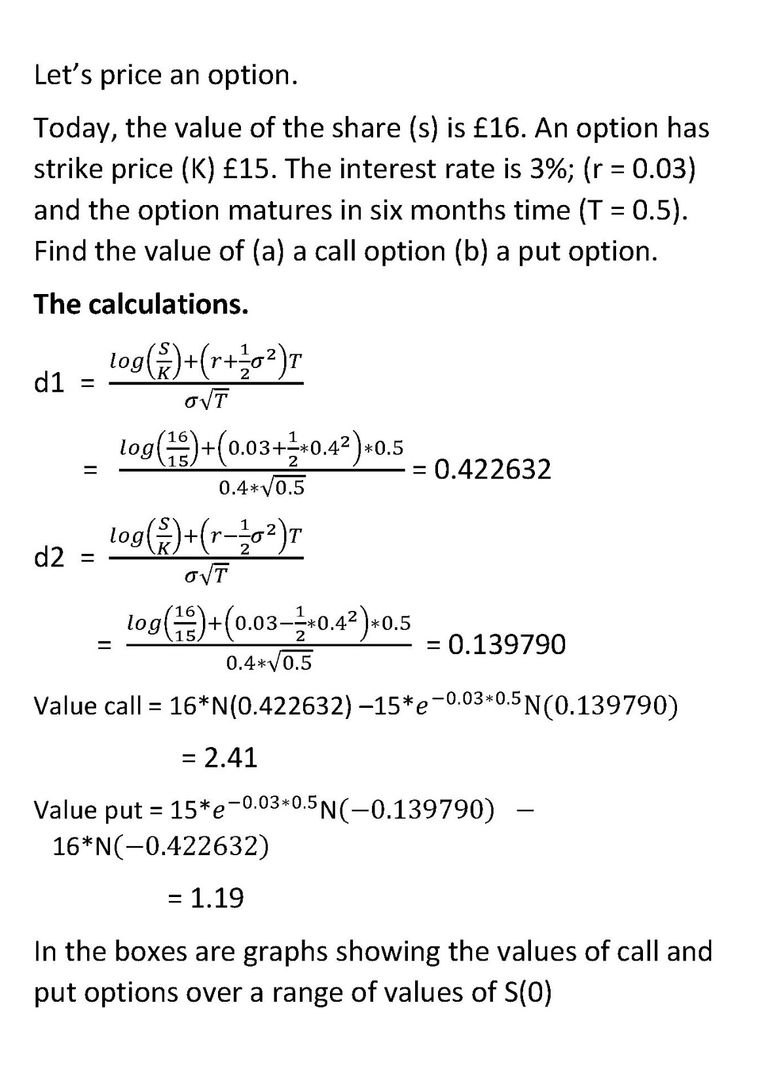
OK. I love mathematics. My interest at the moment is the Black Scholes option pricing methodolgy,
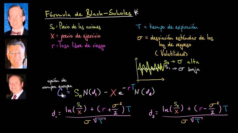
In 1973, Fisher Black (left, below) and Myron Scholes (centre) discovered how to price an option. Robert Merton (right) revealed another way of arriving at this result: his methods permitted a wide expansion of the Black-Scholes result. Sadly, Fisher Black died in 1995. In 1997, Scholes and Merton shared the 1997 Nobel prize in Economics.
The mathematics involved is one of those rare meetings of the seriously useful and the inherently beautiful.
The aim of all that follows is to describe and illustrate the Black Scholes pricing method.


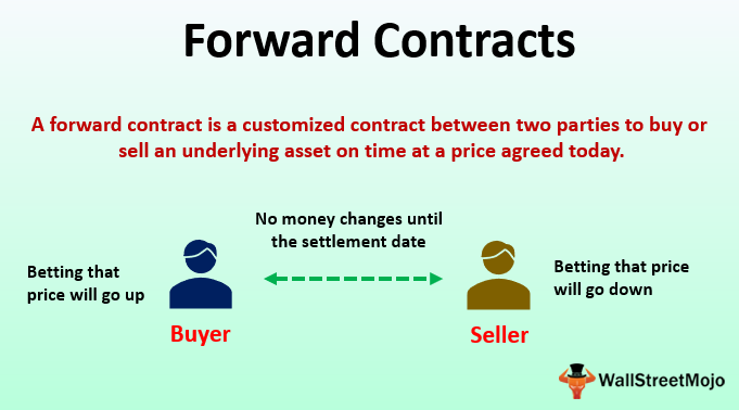
Let's begin by having a look at a forward contract
This morning, I woke up with the thought that over the coming months, the price of AAA shares would rise significantly. I entered a contract to buy, in six months time, 1000 AAA shares at $12 a share.
I pay nothing today. This contract determines that on an agreed date, six months from now, I will buy 1000 AAA shares for $12000. The other party to the contract will, on this date, sell 1000 AAA shares for $12000.
Clearly, if in six months time, the share price is greater than $12, I make a profit. (A share price of $15 would mean that I paid $12000 for an asset worth $15000). If the share price is below $12, I make a loss.
In general terms
In a forward contract, two parties agree that on a named date, a specified asset will be bought/sold at an agreed price. It costs nothing to enter a forward contract. Whatever the value of the asset at the maturity of the contract, the contract must be honoured. A long contract involves buying the asset; in a short contract, the asset is sold.
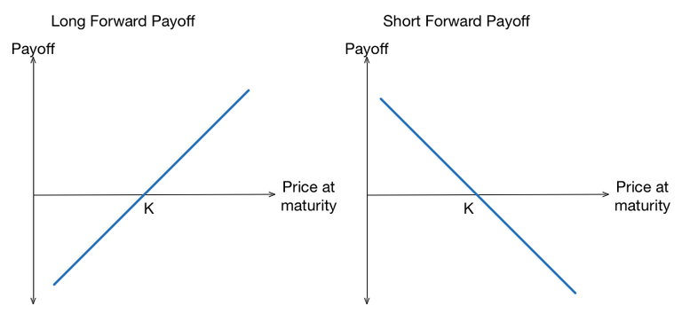
The diagrams illustrate the pay-off from (on the left) a forward contract to sell the asset and (on the right) a forward contract to sell an asset.
But now, a financial anxiety. As the girl on the right explains, "An event which allows for the possibility of unlimited losses is not, in general, a good thing"
And from the above diagrams, it is clear that the potential for unbounded losses exists with both long and short forward contracts. What was urgently desired was a product that allowed a commodity to be bought or sold but where that long potentially damaging tail into negative territory was reassuringly absent.
Enter call and put options.

But first, two bits of 'house keeping'.

A principle
Arbitrage Opportunities
An arbitrage opportunity is a situation which can be used to generate a guaranteed, risk free profit.
It is a principle of financial mathematics that arbitrage opportunities do not exist.
[If an arbitrage opportunity did arise, it would be spotted very quickly by hundreds of hawk eyed traders. They would exploit the situation and by so doing, remove the in-balance in pricing that lead to the arbitrage opportunity.]
A useful technique
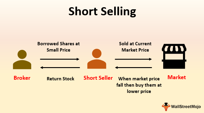
Short Selling
This is the deal. A hedge fund believes the value of an asset (a share, a currency) will fall. In a short sale, the hedge fund will 'borrow' the asset (from a stoke broker) and sell it (short the asset). Later, the hedge fund will buy the asset in the open market and 'return' it to the stockbroker. (close out the sale) IF - as expected - the value of the asset has fallen, the hedge fund make a profit. Otherwise, a loss.
Short selling is tightly regulated and controversial. It is used widely in finance - and is a very helpful concept in pricing theory.
A call option.
The idea is similar to that of a Forward Contract. An investor wants to buy an asset on a given date in the future. Today, that date (the maturity of the contract) and the price the investor will pay for the share, (the strike price) are agreed.
At maturity:
* Forward Contract: the investor has an obligation to pay the agreed price to the other party. The other party has an obligation to hand over the asset.
* With a Call Option, the investor has the right, but not an obligation to full-fill the terms of the contact; that is, to buy the asset, at maturity for the amount given in the strike price. This distinction is critical. If market conditions move against them, the investor can simply 'walk away' and ignore the terms of the contract. (The other party, however, has an obligation to sell the asset at the agreed price if the investor decides to exercise the contract)
Clearly, the holder of a call option has greater freedom than the holder of a Forward Contract.
The asset could be a share, a barrel of oil, a bushel of wheat - almost any traded commodity. We shall mostly assume the asset is a share and write this as S or, if we wish to indicate the time, S(t).
We shall write the time of the maturity as T. The share price, at maturity, will be S(T).
The strike price and will appear as the letter K.
Illustration.
An investor has the idea that in six months time, the price of an AAA1 share will be significantly higher than the present value of £30. There are several things she could do. Two courses of action would be:
[1] Enter a forward contract to buy 1000 shares in six months time at £30 per share. If her hunch was correct and and in six months time, the share price is well above £30, she makes a profit. If the price is below £30, she makes a loss. If the share price crashes, she is obligated to buy 1000 almost worthless shares at £30 a share.
[2] Take out a call option on the share with a strike price of £30 and a six month maturity. If share price rises over these six months, again, she makes a profit. If, however, at maturity, the share price is below £30, she exercises her right to walk away from the deal and does not buy the shares, no doubt breathing a sigh of relief that she chose a call over a forward contract.
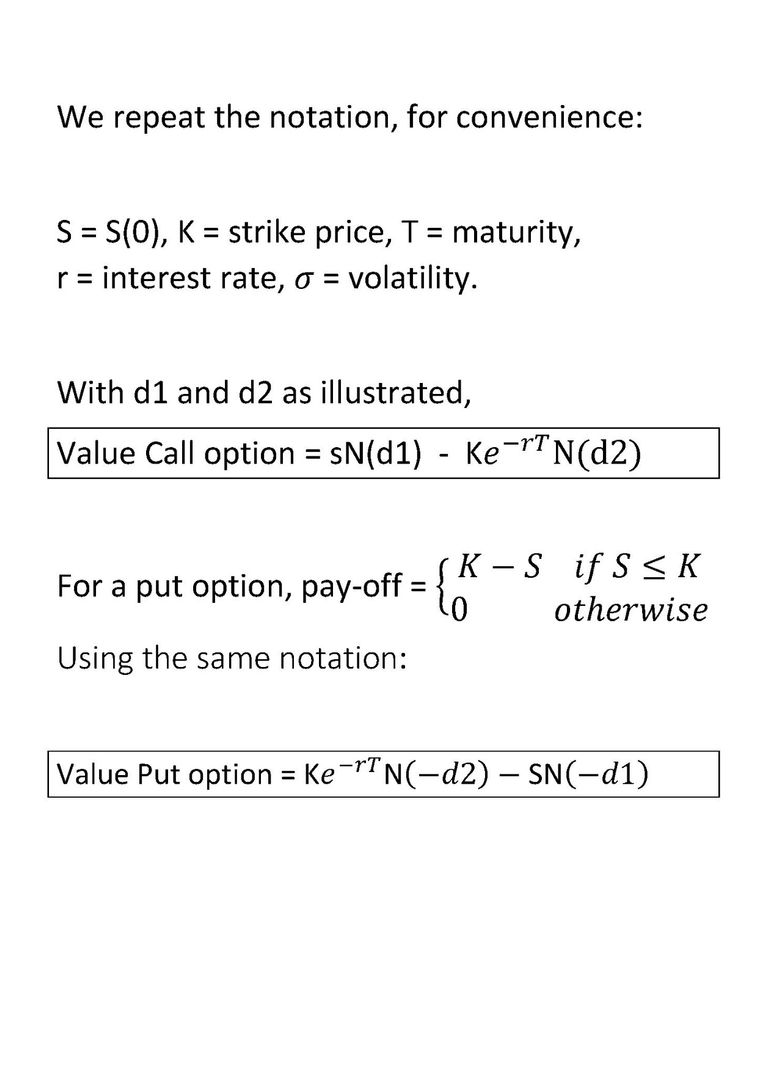
A put option has a structure similar to that of a call option. The only difference is that the holder of a put option is contracting to sell an asset for the strike price at the maturity of the contract. An investor might enter a put option if they felt that value of the asset would fall prior to the maturity.
But: there is a problem here. It appears that a person taking out a call (or a put) option cannot lose money. They can make money. If, at the maturity of a call option, the value of the share (S) exceeds the strike price (K), by exercising the option, they take home S - K. The holder makes a profit while the other party, of course, makes a loss. But if the share price at maturity is less than K, rather than make a loss of K - S, the investor walks away. The other party fails to make the profit they might have hoped for. So it would appear that the holder of an option cannot lose money while the other party to the contract, can. This situation is, to put it mildly, unrealistic. The contract must be, on some level, fair to both parties. To restore a sense of financial equilibrium, the investor will pay a sum of £C to the other party when entering a call option. And similarly, when entering a put option. Now, if an investor 'walks away' at maturity, they will experience a loss of £C. While swallowing their disappointment, the investor might reflect that it is worth paying out a known amount, C to avoid the possibility of unbounded loss.
On the next page, we present diagrams illustrating the pay-off at maturity and profit diagrams for call and put options.
Call and Put options
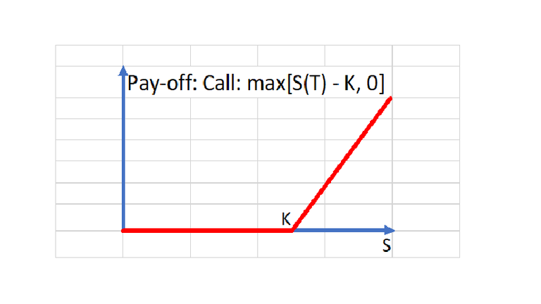
A call option, at maturity.
At the maturity of the contract, (which occurs at time T), the pay-off is as shown above. If, at maturity, the share price is greater than the strike price (K), the option is exercised and the holder buys a share worth S(T) for the lower price, K. If not, the holder walks away. Her payment, at maturity, is £0.
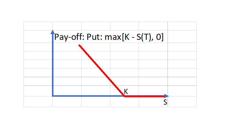
A put option, at maturity.
The graph above shows the pay-off at the maturity of a put option. If the share price at maturity is less than the strike price, the holder will exercise the option and sell a share worth S(T) for the higher value K. (Pay-off = K - S). If at time T, the share price is greater than K, the holder walks away. Their payment, at maturity is £0.
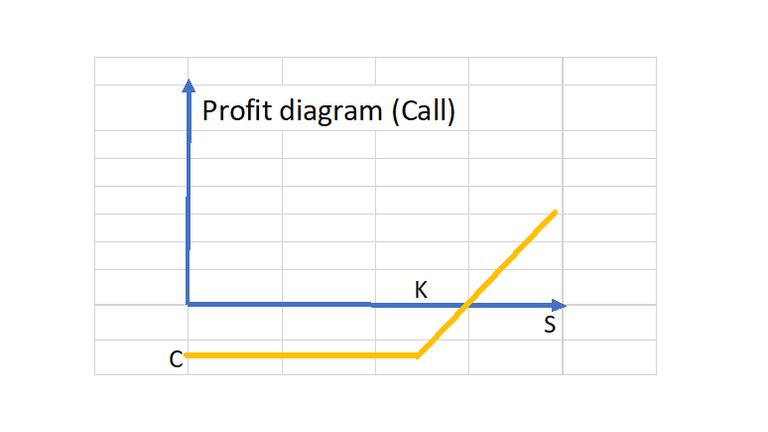
A call option; profit diagram
The investor pays £C to enter a call option. If, at maturity, the share price exceeds the strike price, her profit (S -K) is reduced by £C. If, at this moment, S < K and she does not exercise the option, her "profit" is a loss of £C.
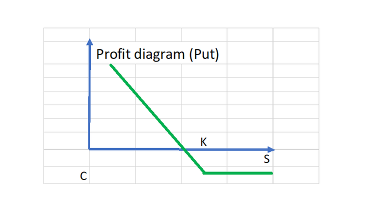
A put option; profit diagram
With a put option also, if the option is exercised, (S(T) < K), the profit is reduced by £C. If S(T) > K and the option is not exercised, the investor will walk away with a loss of £C, the cost of entering the option.
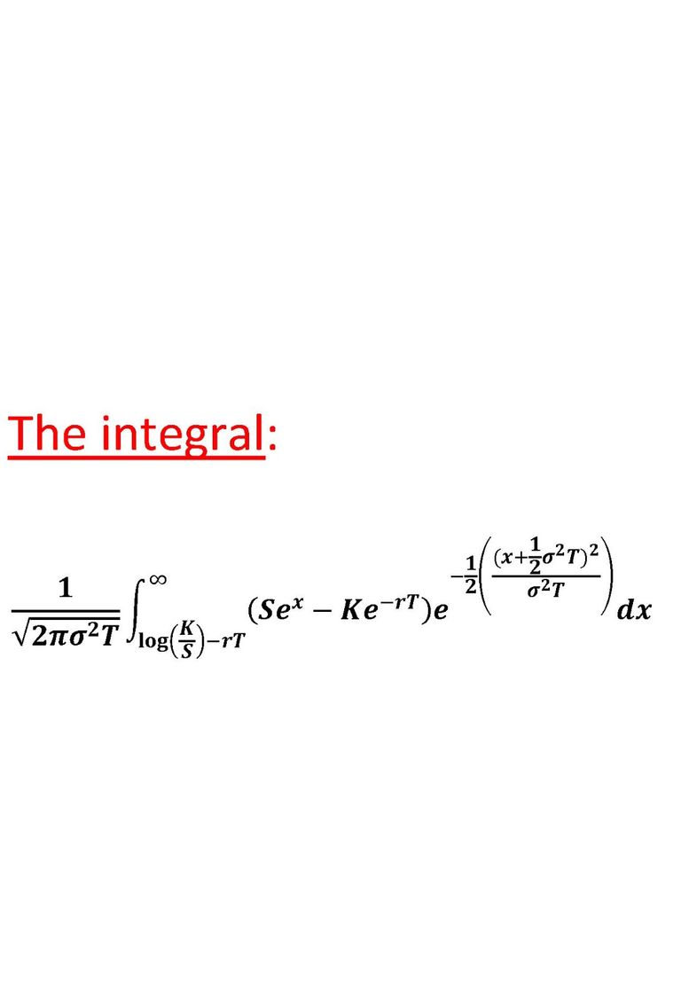
What would be a fair and enforceable value for C?
Now we come to the crux of the matter. Is there a value for C that is fair to both parties? It was for answering this question that Black and Scholes are justly famous. Before we can move towards an explanation of their answer, we must develop ideas in four areas:
[1] we shall need a realistic model for the behaviour of the underlying asset (the share).
[2] we need to understand how interest rates work and how they can be accomodated in our program.
[3] what is an "expected value"? Linguistically, an "expected value" might be what we are looking for. So what is it, mathematically?

[1] We need a sensible and a believable way to model the behaviour of the underlying asset: in our case, a share.
In each figure below are shown three sample paths. The first (top left) shows three Brownian Motions. The other two figures illustrate how these Brownian Motions can be transformed to accommodate certain beliefs in how the share price might behave in practice.

Brownian Motion W(t)
[1] Three sample paths of a Brownian Motion. Each path starts at zero.
Problem. We would like to introduce some reality by being able to represent a possible trend in the share value and market volatility.
A first thought. Try:
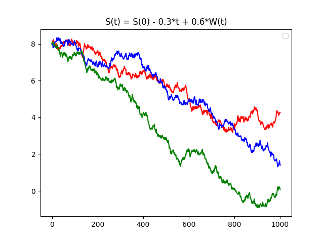
S(t) = S(0) - 0.3*t + 0.6*W(t)
[2] Here, we have a downward trend (-0.3t) and a volatility of 60% - appearing as 0.6*W(t).
Problem. It is possible (see the green path) for the proposed share value to go negative. In any reasonable model, the share value must remain positive.
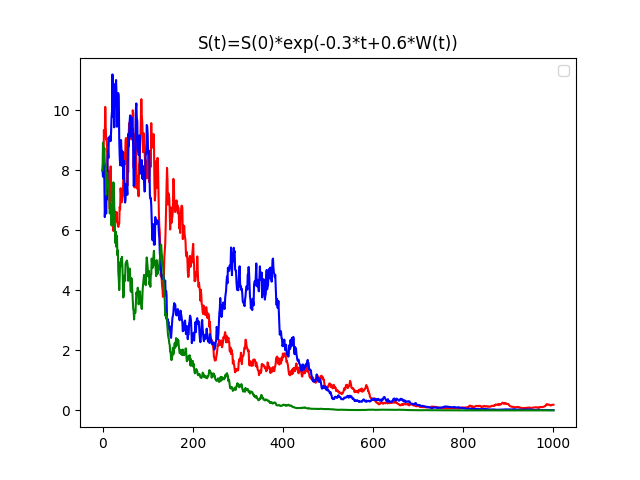
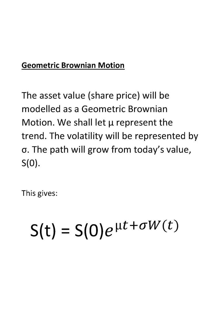
Geometric Brownian Motion
[3] To remove the possibility of a negative value (while retaining the opportunity to represent trend and volatility), express the share value as a power of the constant e (=2.71828182...). By raising e to the power -0.3*t + 0.6*W(t) and introducing the initial value S(0), we get the three graphs shown above. Note that while the green graph (in [2]) goes negative, the green graph in [3] remains positive.


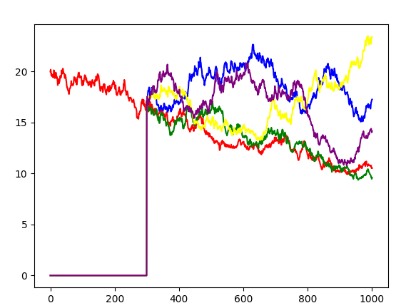
The graphs illustrate the idea. We have shown two paths to t = 300. E[t] is the expected value of the discounted pay-off given knowledge of the path prior to time t.

It's a fair question. Here is the suggestion:
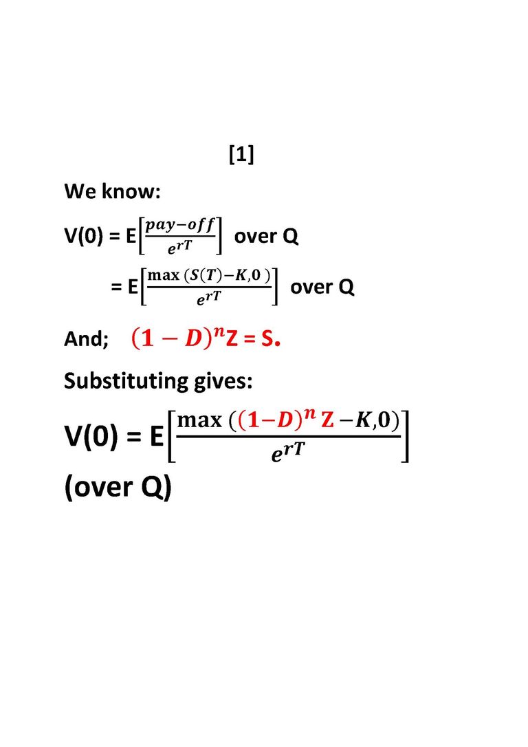
Value of option, today = E[discounted pay-off]
Before we invest hard cash in this suggestion, we need some evidence that it is correct. Such evidence could be provided by a hedging portfolio. This would be a portfolio of traded assets. We will have some units of the underlying asset, S(t) and, to reduce risk, some units of the risk free cash bond B(t).
Let's have, at time t, a(t) units of the share and b(t) units of the cash bond. This would give the portfolio (at time t), a value of:
V(t) = a(t)*S(t) + b(t)*B(t)
The idea is that this portfolio will match, seamlessly and at all times, the value of the option. We need two things to happen.
(i) At maturity, V(T) = X (at maturity: portfolio value = option value)
(ii) The portfolio is self-financing. This means that all changes to the values of S and B are financed entirely from within the portfolio. If the portfolio needs more units of the share, units of the bond are sold to finance the purchase. If the portfolio needs fewer units of the share, the cash from the sale of the surplus shares is invested, in its entirety, in units of the bond. And similarly with any changes needed in units of the bond. Critically: after the portfolio is set up and prior to maturity, no cash leaves the portfolio: no external cash is invested in the portfolio.
Under these conditions, at all times, the value of the portfolio will match, precisely, the value of the option. To see this, suppose that at some time, the portfolio value was greater than the option value, then:
An investor could (short) sell the portfolio, buy the option and invest the excess at the safe rate r.
At maturity: sell the option and use the money to buy the portfolio (at maturity, their values are equal). Return the portfolio (close out the short sale) and withdraw the cash from your investment. This will give the lucky investor a guaranteed, risk free profit. It's an Arbitrage Opportunity. We are agreed. Never going to happen.
Similarly, if at some time, the option value was greater than the portfolio's value.
We conclude: throughout the life of the option: portfolio value = option value.
It would appear that all we have to do to find value of the option at t = 0 is: find the value of the portfolio, V(0), at t = 0.


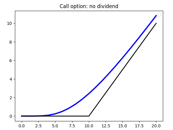
Call option, K = 10
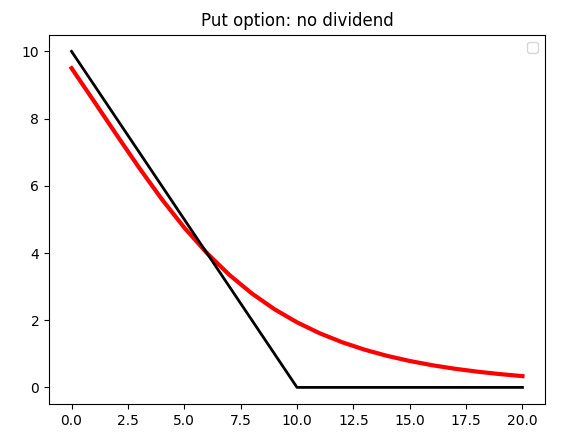
Put option. K = 10
Dividends
Almost all shares pay a dividend. Dividends are paid to shareholders usually either annually or twice yearly and are formed as a given percentage of the share value immediately before the dividend is paid.
To illustrate: let's say that a dividend of 8% is declared to be paid twice yearly. So a dividend of 4% will be paid every six months. Just before the dividend date, the share is trading at £20.50. The dividend, on this occasion, will be £0.04*20.50 = £0.82. To aid discussion, some notation will be useful. Immediately prior to a dividend payment, we write the share value as S. The dividend percentage, as a decimal, is D. The dividend will be D*S. [D=0.04, S=20.50]
We will investigate:
[1] How the payment of a dividend influences the share's value.
[2] How the option price responds to a dividend payment.
[3] How we can navigate a path back to familiar territory.
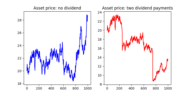
[1] What happens to the share price when a dividend is paid.
Suppose an investor bought a share for £20.50 just before a dividend date. As above, the dividend is 4% so holders of this stock will be paid £0.82 per share. Suppose also that on dividend day, the investor sells a share. If the share price remains at £20.50, the investor will make a guaranteed, risk free profit of £0.82 per share. Never going to happen: see section on Arbitrage Opportunities. To avoid this situation, the share must fall in value by precisely £0.82. To fall by more (or less) would allow an Arbitrage Opportunity. On payment of a dividend, the share price will fall in value precisely by the amount of the dividend.: in this case, by £0.82, leaving the value of the share, post dividend, as £19.68.
This is illustrated in the figure below (where an overly generous dividend percentage has been proposed, to illustrate the share activity.
Using our notation, the dividend payment is D*S and the post dividend share price is:
S - D*S = S*(1 - D)
[2] What happens to the value of the option
The option value depends on time and the current value of the share. To eliminate a riskless profit opportunity of the type described above, the option value immediately pre-dividend must match the option value immediately post-dividend. The holder of the option receives no part of the dividend payment: that goes, in it's entirety to the shareholder. Suppose just after the dividend was paid, the option value were to fall. An investor could (short) sell the option just before the dividend date and buy it back, immediately after, thus making a guaranteed, risk free profit and So we have:
Option value(immediately pre-dividend, share price = 20.50) = Option value(dividend date, share price = 19.68)
This might seem slightly odd. All that has happened is that, as a function of time, the option value has glided across the dividend date unchanged. As a function of the share price, there has been a discontinuity. The effect of the discontinuity in the share value is to make the Black Scholes methodology inadmissible. Which is unfortunate. The Black Scholes formula is a useful device: one we should be reluctant to discard. So I hope you will be pleased to learn that mathematicians have found a way round this local difficulty - at least, when the dividend date and the dividend percentage are "known". The idea is simple, but surprising in it's effectiveness.
[3] Navigating a path back to Black Scholes.
This is the plan. Set up a new portfolio consisting solely of units of the underlying share. Call this portfolio, Z. Construct Z as follows:
Initially, Z will contain one share. So until the first dividend payment, Z and S will share a common value.
On the payment of each dividend, use the money released to buy more units of the underlying share and accommodate these additional shares in Z. In a sense, the share value that was lost to S, - with the payment of a dividend - has been recovered in Z.
By this arrangement, post dividend, Z has the value S would have had if no dividend was paid.
So Z*(1 - D) = S (where S represents the post dividend share price.)
If there is a second dividend, the procedure will give Z*(1 - D)*(1 - D) = S. And so on, with further dividend payments. From the construction, S has jumps, Z does not. Because of these jumps, an option based on S will not fit into the Black Scholes framework. However: an option based on Z, will.
How does this work, in practice?
Four sections explain the method
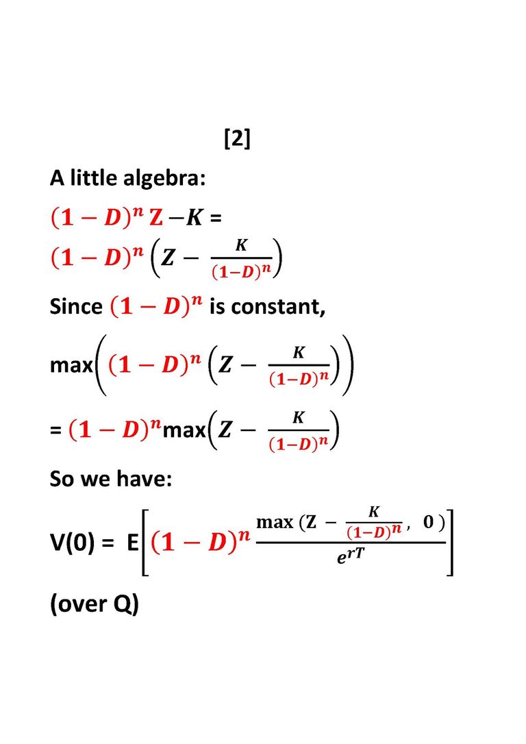


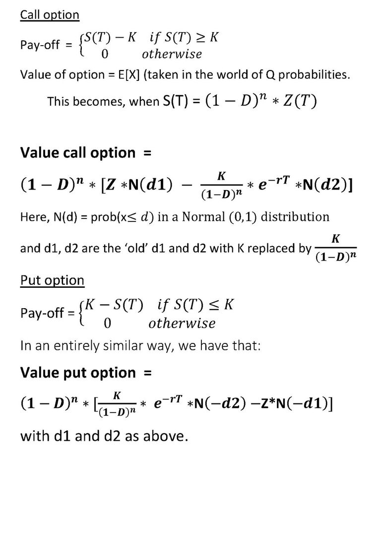
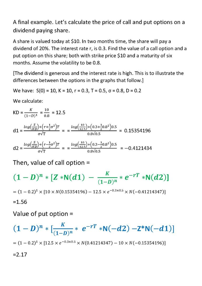
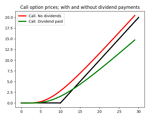
The Black Scholes type formulae applied to the Expected Value of the Z function. Observe the 'new' strike.
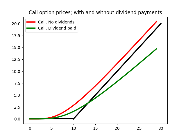
Values of a call option with strike K=10. Rate = 0.3, sigma = 0.8, T = 0.5
One dividend payment with D = 0.2

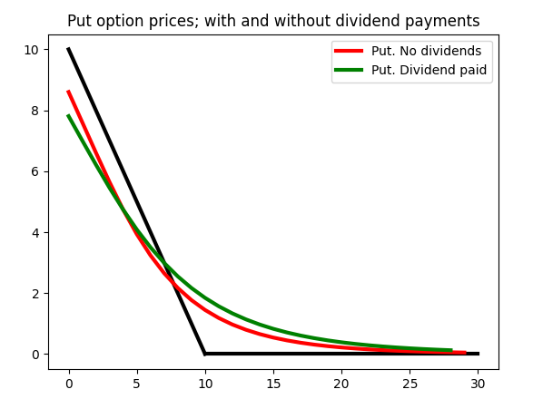
Values of a Put option; data as above.
A brief history of options
Thales (4th century BC)
Russell Sage (1815 - 1906)
There were four significant moments in the development of options.
Thales of Miletus (4th century, BC)
Thales was an astromoner and from his observations of the stars, came to believe the next olive harvest would be plentiful. Hence, there would be a healthy demand for olive presses. Thales paid olive press owners to secure the right to used their presses at harvest time. There was, indeed, a huge harvest that year. Thales then re-sold the rights to these presses and made a timely profit! He had bought the right to use the presses: not an obligation. He demonstrated also that options can be profitably traded.
A tulip mania in Holland in the 17th century.
Unlikely as it seems, in 1634, Holland experienced a market bubble in, of all things, tulips. There was a tulip mania with the price of some bulbs rising astronomically. Tulip growers wanted to protect their profits against against falling prices; they bought what amounted to put options. Wholesalers, on the other hand were afraid of a rising price: they protected their positions by buying call options. So options can be used as insurance against adverse market conditions. (This is known as 'hedging')
Russell Sage: late 19th century
In the late 19th century, Russell Sage (pictured above) created options that could be traded. These were 'over the counter' trades, largely unregulated. Sage was the first person to exhibit a relationship between the price of the option ($C), the value of the underlying asset and interest rates.
Chicago Board of Options Exchange, 1973.
The year 1973 was a good year for options. The Chicago Board of Trade, in 1973 opened The Chicago Board of Options Exchange (CBOE). Options were now standardised and for the first time, were traded on an established exchange.
Just as important: this was the year in which Black and Scholes published their epoch making formula allowing, for the first time, the value of an option to be calculated.
References
Financial Calculus, Baxter and Rennie,
Cambridge University Press, 1996
Financial Products, Dalton
Cambridge University Press, 2008
A Course in Financial Calculus, Etheridge
Cambridge University Press, 2002
If the references have appeared, it must be The End. And it is - of this presentation.
I hope you have enjoyed seeing some of the marvellously creative thought that has gone into pricing options.
The next step (for me) is to understand option pricing when the asset is subject to unpredicatable jumps. The layers of uncertainty, in finance as in life, just keep on building. Goodbye. Thank you for reading this.
© Copyright. All rights reserved.